Circuiting Done Right

When designing a new injection mold, a moldmaker’s main goal should be to put its client in the best position to make quality parts consistently and efficiently.  A significant part of that is the cooling design, where there are many things to consider, most of which are crucial to the operation of the mold.  Getting the most out of a cooling design involves figuring out how to get around obstacles such as melt delivery systems (hot runners, cold runners, gates), part ejection, and mold action (slides, lifters).  These obstacles can usually be overcome by using sound mold design principles, cooling simulation and some creativity.  But cooling a mold uniformly isn’t just about getting the cooling lines in the right place.  It also requires supplying the right amount of water, effective circuiting and using simulation to get it right—the first time.  

“Cooling analysis will reduce cycle times by 8-10%.”

In a previous article (MMT, January 2013), we talked about using flow simulation to help determine the best gate locations and how to size them properly.  Did you know that the cooling process can also be simulated?  The process is very similar to flow simulation, only now we’re putting cooling lines in the right place, instead of gates.  And just as with flow simulation, cooling simulation must be done properly and in a timely fashion in order to have the greatest impact on the mold design.  Thus, cooling simulation is best left in the hands of engineers with years of experience using the software to analyze injection molds.  

Cooling analysis done properly provides uniform cooling, reduced cycle times and efficient coolant management before you find out too late that you have problems at the press.  We’ll address only the coolant management here.

Suppose you are already convinced that you have a great cooling design.  You used simulation to optimize your cooling line locations or to figure out where a beryllium copper insert was needed for a difficult area to cool.  Wouldn’t you be disappointed if it all got blown up at the press simply because the processing team failed to plumb the mold effectively?  It probably happens more often than most people in the industry care to admit.  You don’t have to visit too many molding shops before you notice that circuiting cooling lines is often an afterthought.  Looping too many lines together or providing an inadequate amount of water can result in cooling lines that have excessive temperature rise.  That rise in temperature can turn what should be uniform cooling into non-uniform cooling, which can cost you cycle time, or even worse—part quality.

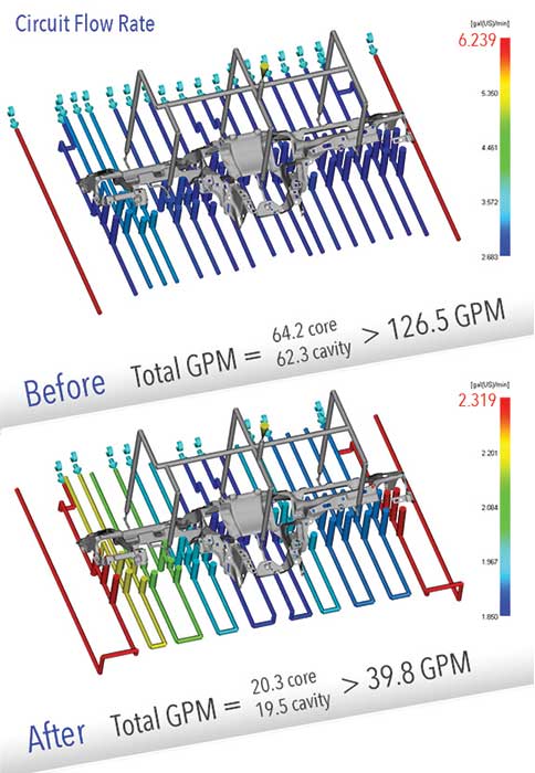
Cooling simulation will help you avoid this problem by pinpointing exactly which lines are good candidates for looping together.  Circuiting done properly allows the cooling lines to share water without compromising cooling uniformity.  This is particularly important for larger molds where having enough GPMs becomes a concern.

Selecting Cooling Lines for Looping
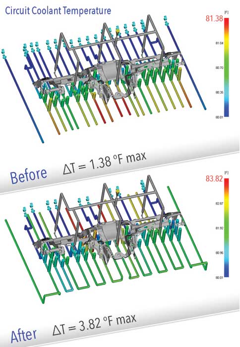
So, what is the right way to circuit cooling lines?  After determining the best cooling line locations and approximate cooling time, the analyst turns his attention to the coolant flow.  The analyst’s goal is to achieve turbulent flow in all channels while maintaining a temperature rise (ΔT) in the coolant that is less than 3-5°F—preferably closer to 3°F.  Turbulent flow provides efficient heat transfer; controlling the ΔT prevents hot spots in the mold due to hotter water.

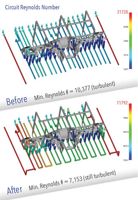
It is best to analyze each line individually so that their ΔT’s can be determined.  The analyst must establish turbulent flow and then find good candidates for looping.  First, we’ll talk about turbulent flow.  It is imperative that turbulent flow is achieved in each of the cooling lines because heat transfer rates between the water and mold steel are optimal when the water is turbulent.  Turbulent water provides roughly seven times the heat transfer rate of the alternative—laminar flow.  So, providing turbulent flow means faster cycle times.

“Turbulent flow is a key factor in cycle time reduction.”

But what is turbulent flow, and how do you know the molder can achieve it?  Oswald Reynolds developed an equation for what he called the Reynolds Number (Re) by studying fluid flow in pipes.  It is based on the relationship between dynamic pressure and shearing forces within the flow.  The equation can be written in several ways, but the most useful for injection molding is:

Re=  (3160 Q)/(D η)
Re=Reynolds number
D=diameter of cooling channel in inches
Q=flow rate in GPM
η=kinematic viscosity in centistokes

Reynolds differentiated between laminar and turbulent flows in his equation by saying that turbulent flow is achieved when the Reynolds number reaches approximately 4200.  The problem with laminar flow is that the coolant flows in layers, which reduces heat transfer between the coolant and the steel and increases the temperature of the coolant nearest the steel.  This sets up a lower temperature differential between the coolant and the plastic, which in turn slows the removal of heat from the mold.

The simulation software handles the Reynolds number calculations after the analyst inputs the water temperatures and pressure conditions at the inlets to each channel.  If the analyst knows ahead of time how many GPMs will be available for a particular molder, that information can be input into the simulation instead, and the software will calculate how much flow each cooling line will get.  

Once the flow rates and heat transfer rates are calculated, the ΔT’s are reported and the analyst can choose which lines will be looped together based on the following criteria:
    ΔT < 1°F
    Cooling lines are in close proximity
    Cooling lines are the same diameter

It is often the case that a cooling line will have a very low ΔT, which usually means it also has a high GPM rating.  These can often be looped together in a series of three or four lines without exceeding the ΔT criteria.  A tremendous amount of GPM can be saved in this case.

Shown in the graphics is a before and after case for circuiting.  As you can see, there was a significant reduction in the amount of water required after circuiting, yet turbulent flow was maintained, along with acceptable ΔT’s (see Figures x – x).

There are a couple of ways to implement the circuiting recommendations—internally or externally.  Circuiting/flow diagrams should be provided for each mold.  If possible, internal circuiting should be used because it reduces the amount of plumbing that needs to be done at the press.  There will also be less possibility of misinterpreting the circuiting instructions.

There is also another possibility—flood cooling.  If the GPMs are adequate to supply the cooling lines uncircuited, then each of those lines can be connected to a large supply and return line.  Be careful where you place the inlets and outlets or else some of the lines will receive more flow than the rest.

Summary
Making the investment in cooling simulation with a qualified, certified analyst will help you make better molds and will set up your customers to mold quality parts more consistently and efficiently.  And that will help you win more business in the long run.  Remember, it’s not just the placement of cooling lines that matters, it’s also important to get the circuiting right.